Open Boundary Conditions#
In transport simulations, we are modeling driven quantum systems. This means that charge carriers are injected into the considered simulation domain from one contact, and they are extracted from the domain at another contact. Since we have to restrict the part of the system that we model explicitly, these contacts are approximated as semi-infinite reservoirs in thermodynamic equilibrium that are connected to the simulation domain and can provide or absorb charge carriers. As long as the contacts are sufficiently far from the active region of the device, these equilibrated reservoirs are usually a good approximation.
Figure 1. Device with semi-infinite contacts, where charge carriers are injected and extracted. The contacts enter the transport equations through the open boundary self-energies.
In quatrex, the electronic structure of the contacts is extracted
directly from the provided Kohn-Sham Hamiltonian and overlap matrix. The
contact matrix elements are selected based on the geometry of the system
and the provided configuration.
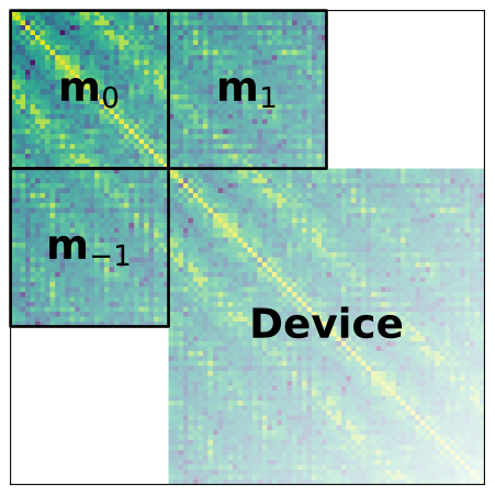
Figure 2. The left contact blocks of the carbon nanotube system. For this example, the contacts are simply the left- and right-most blocks as the system is created by repeating the Wannier centers.
Since these open contacts can be understood as "renormalizing" the dynamics of the closed system, they enter the quantum transport equations through the retarded and lesser/greater open boundary self-energies \(\mathbf{\Sigma}^{R}_{OBC}\) and \(\mathbf{\Sigma}^{\lessgtr}_{OBC}\), respectively.
Retarded Open Boundary Self-Energy#
The retarded boundary self-energy \(\mathbf{\Sigma}^{R}_{OBC}\) can be calculated from the retarded surface Green's function \(\mathbf{g}^R\) through the following equation:
Since we assume that each layer in our contact has the exact same electronic structure and sits at equilibrium, we obtain \(\mathbf{g}^R\) from the following fixed-point problem:
This problem can be solved with different methods, which will be discussed below. As illustrated in Figure 2, \(\mathbf{m}_{0}\) is the layer's system matrix contact block while \(\mathbf{m}_{1}\) and \(\mathbf{m}_{-1}\) are coupling blocks from the contact to the device (see also the sections on NEGF and QTBM).
In the case of QTBM, the contact blocks \(\mathbf{m}_{x} = E\mathbf{S}_{x} - \mathbf{H}_{x}\) are Hermitian: \(\mathbf{m}_{0} = \mathbf{m}_{0}^\dagger\) and \(\mathbf{m}_{-1} = \mathbf{m}_{1}^\dagger\). This is not strictly the case for NEGF, since the blocks include scattering. Taking electron-electron scattering as an example, the inclusion of \(\mathbf{\Sigma}^R_{GW}\) breaks the symmetry of the contact blocks
Similarly, for the screened Coulomb interaction, the product \(\mathbf{V}\mathbf{P}^R(E)\) breaks the symmetry of the contact blocks:
Lesser/Greater Open Boundary Self-Energy#
When employing NEGF, besides the retarded self-energy, we also need to compute \(\mathbf{\Sigma}^{\lessgtr}_{OBC}\). Since we impose thermodynamic equilibrium conditions at a set temperature in the contacts, in the case of the electronic system, we can get the lesser/greater self-energies via the fluctuation-dissipation theorem, resulting in the following equations:
Where \(\boldsymbol{\Gamma}(E)\) is the broadening matrix, \(f_{FD}(E; \mu, T) = \left[1 + \exp\left(\frac{E - \mu}{k_B T}\right)\right]^{-1}\) is the Fermi-Dirac distribution, \(\mu\) is the contact's chemical potential, \(k_B\) is the Boltzmann constant, and \(T\) is the temperature of the electron occupancy in the contact.
For other interacting systems, like the screened Coulomb interaction, we cannot directly apply the fluctuation-dissipation theorem, since we do not directly control the occupancy of the bosonic modes. Instead, similarly to the retarded self-energy, we can obtain the lesser/greater self-energy in terms of the lesser/greater surface Green's functions, \(\mathbf{w}^{\lessgtr}\), that satisfy a similar fixed-point problem as in Equation \(\ref{eq:obc_recursion}\), but with a different structure. The lesser/greater self-energy is then given by the discrete-time Lyapunov equation (or Stein equation):
This is discussed in more detail in this section, along with different solution approaches.
Solution Approaches#
One can differentiate between iterative and direct methods for solving the fixed point problem of Equation \(\ref{eq:obc_recursion}\). There exist general results on fixed points such as the Banach and Brouwer theorems, but there are limited results that are specific to Equation \(\ref{eq:obc_recursion}\).
Selecting a solution approach
The specific OBC algorithm can be selected through the
algorithm parameter in all
subsystems (Electron,
CoulombScreening,
Phonon, and
Photon).
No iterative solution approaches for QTBM
For QTBM, currently only the direct algorithm called spectral is
available. This is due to the fact that QTBM requires information on
the system's eigenmodes for the calculation of the injection
vectors, i.e., for the assembly of the system of equations.
Iterative#
Generally, iterative approaches are quite simple to implement and typically highly performant from a computational perspective, but they can struggle with convergence. The recursion relation may not reach convergence at all, or it may converge at different rates for different energies. This is especially true for energies close to Van Hove singularities.
Another concern is the choice of a good initial guess for the surface Green's function. A good initial guess can greatly improve convergence, while a poor initial guess can lead to divergence. More on this can be found in the memoization section.
Fixed-Point Iterations#
The most straightforward iterative approach is to perform fixed-point iterations as
If this scheme happens to converge, it does so at a linear rate. Due to
the slow convergence, this method is not directly exposed in quatrex.
Instead the method is only used to refine the solution coming from the
spectral method. Further, it is used in the memoizer
to refine solutions from previous iterations.
Forcing Fixed-Point Iterations
For testing purposes, it is possible to only do fixed-point
iterations in NEGF. This can be done by setting the
mode parameter of the
memoizer to "force".
Sancho-Rubio#
Alternatively to simple fixed-point iterations, the Sancho-Rubio method
is a well-established iteration scheme that accelerates the convergence
of the surface Green's function 1. The method achieves an exponential
convergence rate, but still requires the problem to be well-posed. To
stabilize the method, a small complex value should be added to the
boundary blocks which can be done by setting
eta_obc for the electron solver.
The following other parameters affect our implementation of the Sancho-Rubio method:
Direct#
Direct methods require more care in their implementation and can sometimes be less performant than iterative methods, but they are more robust and can be used for any energy.
Spectral Method#
It can be shown that the solution of Equation \(\ref{eq:obc_recursion}\) can be expressed in terms of the eigenpairs of the polynomial eigenvalue problem
This spectral method is also implemented in quatrex and is the
recommended default. The method consists of two main steps:
- Eigenvalue problem: Solve the polynomial eigenvalue problem with any algorithm.
- Post-processing: Filter the eigenpairs and use them to construct the surface Green's function.
The construction of \(\mathbf{g}^R\) in terms of the eigenpairs is done as
where \(\mathbf{V}\) and \(\mathbf{\Lambda}\) are the matrices of eigenvectors and eigenvalues of Equation \(\ref{eq:poly_eig}\), respectively.
Since only reflected modes contribute to \(\mathbf{g}^R\), the filtering step is essential to get an accurate result. The NEVP page elaborates on the available eigenvalue solvers and on the filtering step. Further details about this method can be found in 2.
Memoization#
Lastly, the memoizer can be used to
accelerate NEGF simulations when there is limited change between
iterations. It works by storing \(\mathbf{g}^R\) of the previous SCBA
iteration and trying to refine it with cheap fixed-point iterations. If
the residual after a single fixed-point step is low enough, the
expensive call to the solver is skipped and a fixed number of iterations
is performed instead. The method can be efficient, but requires a bit
more memory.
Reducing Memory Footprint
We plan to compress the stored \(\mathbf{g}^R\) guess to reduce the memory footprint.
Caution with Memoizer
The behaviour, described above, concerns the (default) "auto"
setting of the memoizer mode.
All other modes (except for "off") should be used with caution, as
they may lead to unstable behaviour. Simulations using
"force-after-first", meaning a single iteration of a real solver
and then always refining, have worked in our experience, but
resulted in OBC convergence warnings which usually stopped after a
few iterations. It is not studied how these different convergence
paths differ.
The memoizer only brings performance benefits if all MPI ranks agree
to memoize. If some energies are not memoizing despite an otherwise
stable simulation, then the
agreement_threshold
should likely be lowered.
Memoizers for both retarded and lesser/greater self-energies
The memoizer is both a member of the OBC and the Lyapunov config
since both are capable of benefiting from memoization. In both, the
memoizer can be separately configured.
-
Sancho, M. P. L., Sancho, J. M. L., & Rubio, J. (1984). Quick iterative scheme for the calculation of transfer matrices: application to Mo (100). Journal of Physics F Metal Physics, 14(5), 1205–1215. ↩
-
Brück, Sascha. Ab-initio quantum transport simulations for nanoelectronic devices. Diss. ETH Zurich, 2017. ↩